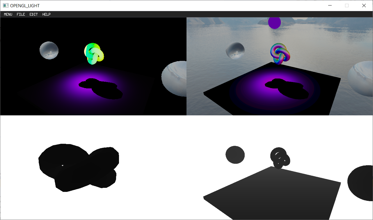
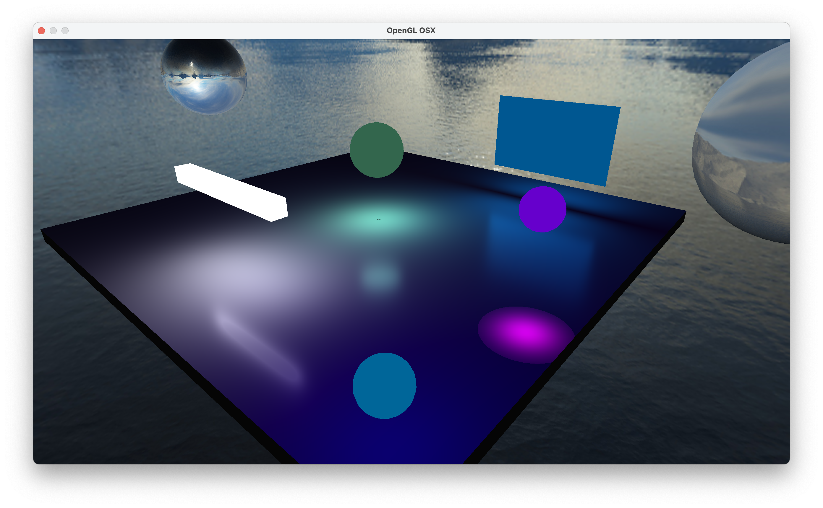
This is a new attempt as the lighting part of the rendering system in my engine program. I have built several common lights in the rendering system. Because it is implemented with OpenGL3.0 and is based on a rasterized rendering pipeline. Therefore, there are still some defects in global lighting.
Concepts
First of all, let’s review some basic concepts.
Radiant Flux : energy per unit time, say it’s measured in watts. Unit is
.
Irradiance : the flux incident on the surface per unit surface area.
Radiant Exitance or
: or called radiosity, the flux leaving a surface per unit surface area.
Radiance : the flux per unit area normal to the beam per solid angle.
BRDF: the bidirectional reflectance distribution function gives a formalism for describing reflection a surface.
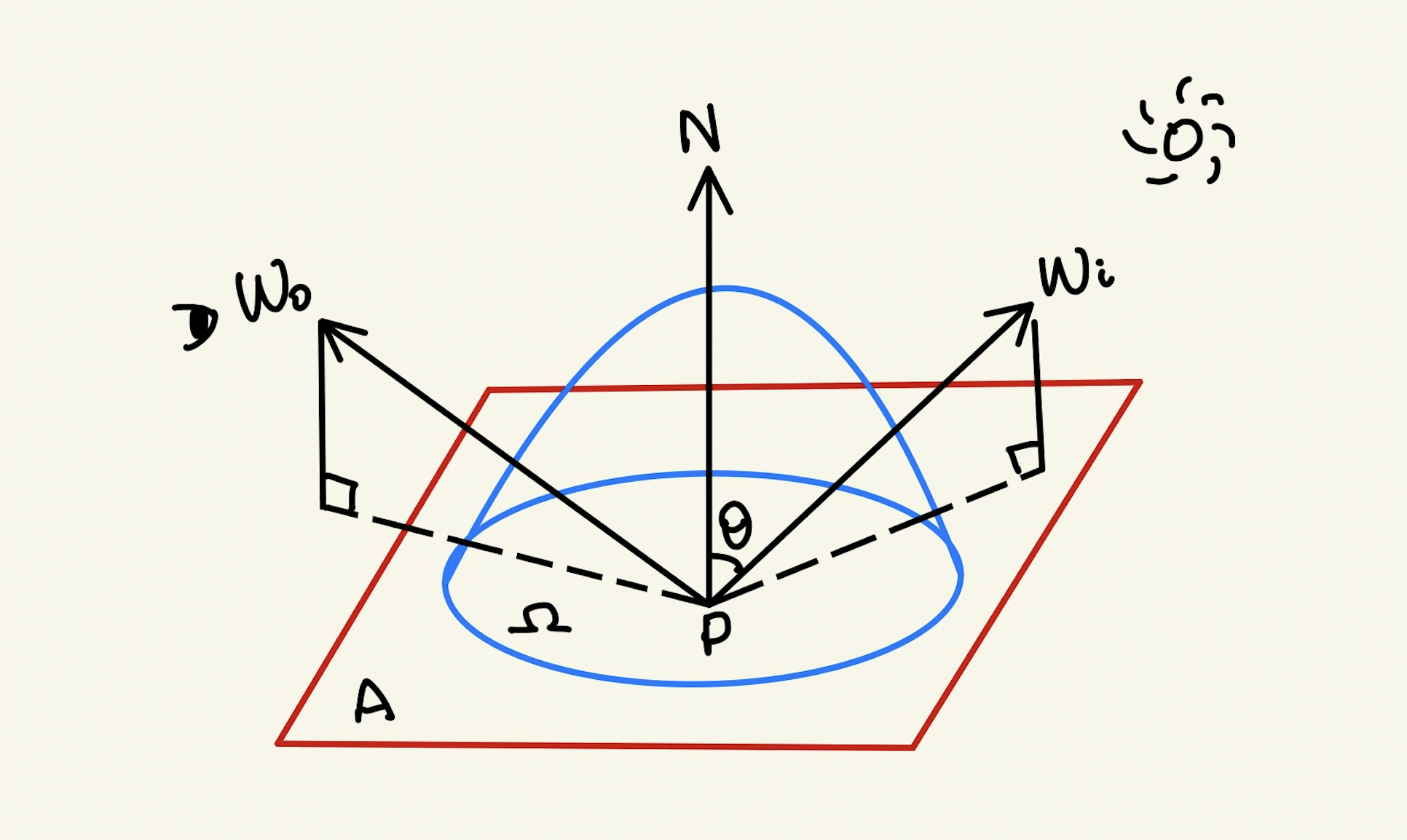
Therefore,
Then,
So,
Finally, a rendering equation is obtained.
Blinn-Phong
1 | vec3 N = normalize(normal); // normal vector |
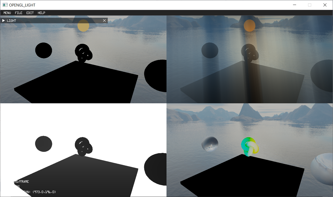
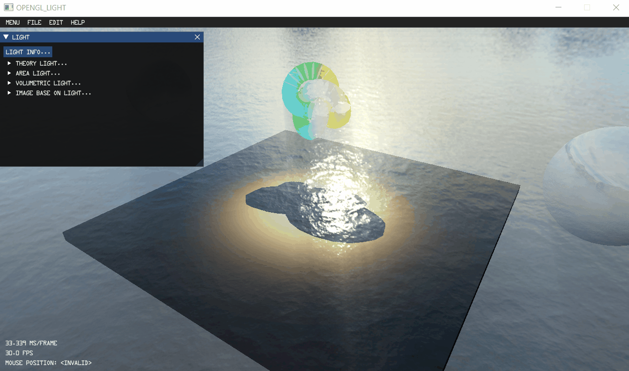
Theory Light
Point LIGHT
The point light source naturally has only one direction for a point with incident light, so there is no integral here. This is also means that it does not need to consider the direction of light, but needs position information.
In addition, it is importance to consider the attenuation for the point light source.
First way
1 | float dist = length(L); |
Second way, Professor Cem Yuksel proposes an attenuation function that considers the radius of light source to eliminate the singularity of the inverse-square light attenuation function.
Directional LIGHT
Compared with the point light, it does not need to consider the attenuation of light and the position information of light, but it need to consider the direction of light.
1 | vec3 L = normalize(light.direction); |
Spot LIGHT
For Spot light, it should consider both the direction of the light and the position information where the light is needed. At the same time, it is necessary to calculate the attenuation factor.
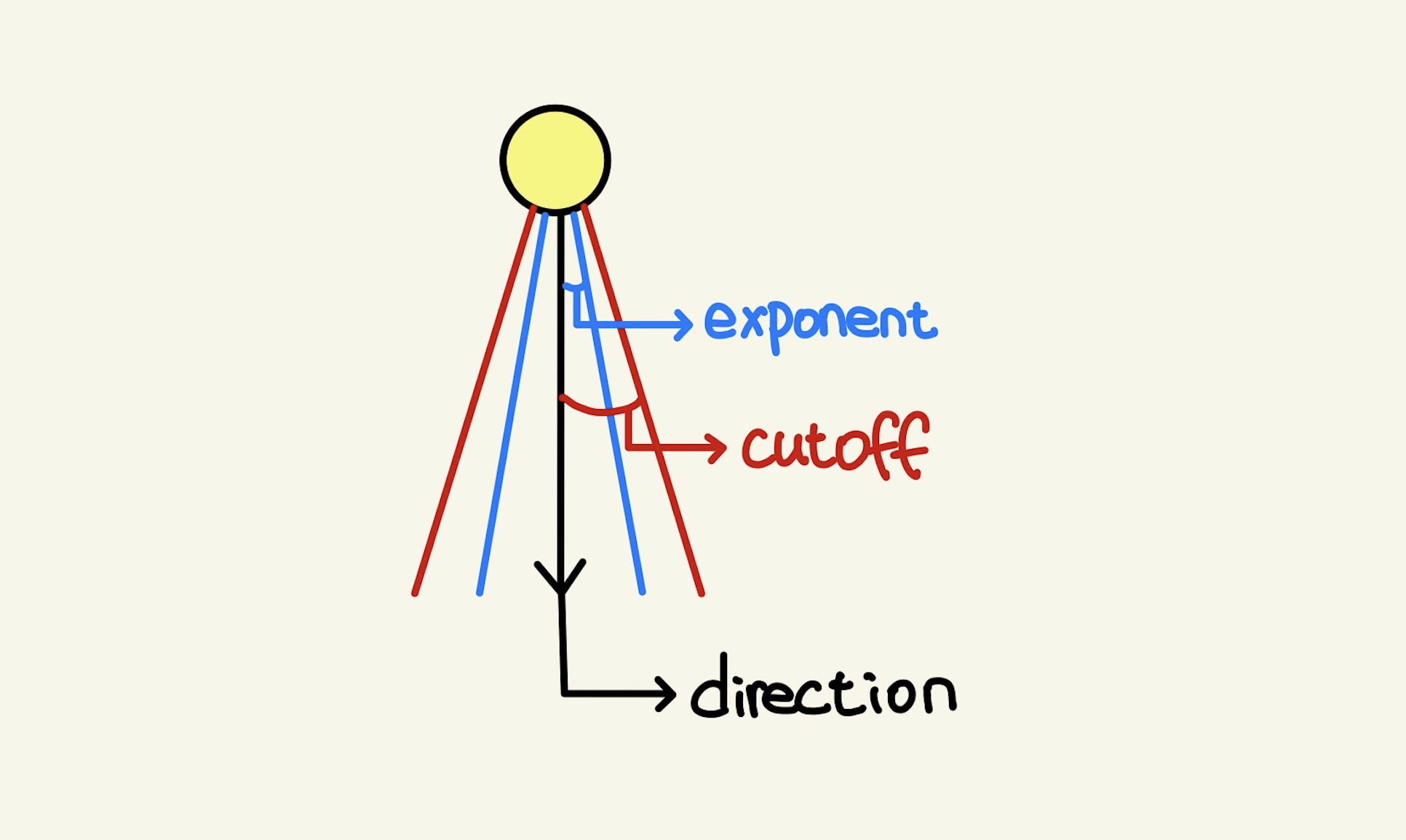
1 | vec3 spotDir = normalize(light.lightDir,xyz); |
Area Light
For the area light source, we can treat it as a set of infinitely many point light source, so we only need to integrate the solid angle range of the area light and determine the radiance of the incident light of the area light source in different solid angle.
In addition, for the rendering equation we discussed earlier, we need to calculate an analytic expression mathematically, but there is no analytic expression for the above integral. Therefore, a well-known method is Monte Carlo.
But it is troublesome to use Monte Carlo. we can directly trick. At the same time, we can use light transport theory to optimize.
Another method is polygonal-light shading with LTC proposed by Eric Heitz et al.
After determine the incident direction and roughness, BRDF become a spherical distribution function. As we said before, the key point problem needs to be solved is analytic expression. Heitz’s paper shows that we can convert the BRDF spherical distribution function into the spherical distribution function of .
In short, we are changing the BRDF linear transformation to a cosine distribution in rendering.
Then, the LTC can be obtained,
Base the GGX BRDF, we can use four parameters to create a M. It is also mean find a LTC.
So, we can store it in a 2D four-channel LUT. According Ubpa’s summary, we can summarize a process.
- Sampling LUT and get M.
- Change the vertex of polygon to the [T1, T2, M] coordinate system.
- Crop polygons.
- Integral.
- Sampling Norm and Fresnel term to adjustment step 4.
 .
.
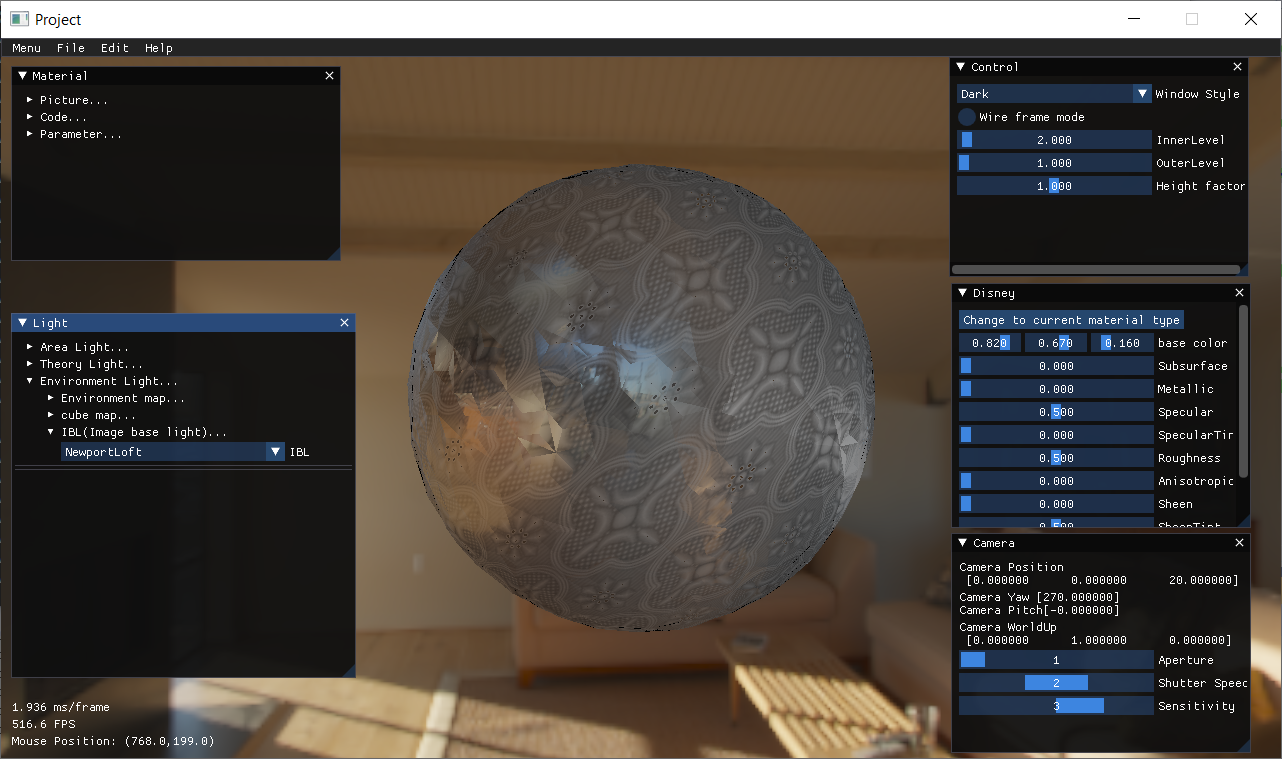
IBL (Image Based Lighting)
IBL is often used in Physically Based Rendering, which uses theory based on physical and microfacet theory to shading and uses surface parameters measured from reality to accurately represent real-world materials. In my view, IBL is an excellent ambient light.
At present, one of the most common models is Cook-Torrance.
In this equation, N means Normal Distribution Function, which is used to describe microfacet normal distribution.
In this equation. F means Fresnel coefficient, which is used to describe reflectivity. The value range from 0 to 1.
Schlick gives simplified definition.
In this equation, G means Geometry Function, which is used to describe geometry obstruction and geometry shadowing. The value range from 0 to 1.
So, update the rendering equation.
This is means, radiance can be obtained by using to sample the cubeMaps.
1 | vec3 radiance = texture(cubeMaps, w_i).rgb; |
So, we calculated through The Monta Carlo integral to get an Irradiance Map. When using the irradiance map, sample according to the normal direction, and multiply to get the diffuse reflection item.
1 | vec3 irradiance = texture(irradianceMap, N); |
Joey gave specific sample codes about Pre-calculation in his book.
1 | vec3 N normalize(worldPos); |
Last, finally, calculate the specular factor.
Epic Games proposes a method called split sum approximation. Therefore,
First, calculate the first integral. Similar to the above method, we can get a Map, which called pre-filter environment map.
1 | float saTexel = 4.0f * Pi / (6.0f * resolution * resolution); |
Second, calculate the second integral. The obtained Map called BRDF LUT. So, the current problem is how to create a LUT Map. According the previous rendering equation, we need four parameters. we can find a way to eliminate $ F_0$.
After that, using Monta Carlo to solve scale and bias. Both parts can represent the pre-calculated results with a 2D texture. They are all 1-dimensional variables that can be placed in the same texture, scale in the red channel, and bias in the green channel. In the end, using (range between 0.0 and 1.0) as the horizontal coordinate and roughness as the vertical coordinate to create a LUT. This LUT is determine by BRDF,so the determined BRDF has a determined LUT.
1 | vec3 IntegrateBRDF(float NdotV, float roughness) |
Now that we have three texture maps, they are irradiance Map, pre-filtered Map, and LUT. we can get the .
1 | vec3 Ks = F; |
 .
.
Volumetric Light
Kenny Mitchell mentioned a method called Volumetric Light Scattering as a Post-Process in the book GPU Gems 3. In short, this method is divided into three steps.
In the screen space, we lack enough information to calculate and determine occlusion. But, we can estimate the probability of occlusion at each pixel by summing samples along a ray to the light source in image space.
In addition, adding attenuation coefficients to parameterize control of the summation.
- Rendering the light source and occluding objects to the framebuffer, which called Occlusion Texture Map. According to the sampling diagram and some light scattering algorithms, the Light Scattering Texture Map can be obtained.
- Clean the depth buffer, render the scene without light source to the another framebuffer, which called Scene Texture Map.
- Switch camera to 2D(Orthogonal projection)
- Blending Scene Texture Map and Light Scattering Texture Map.
1 | void CalcLight() { |
Reference
[1]Philp Dutré,Kavita Bala, Philippe Bekaeert.Advanced Global Illumination.2nd Edition.
[2]Cem Yuksel.Point Light Attenuation Without Singularity.ACM SIGGRAPH 2020 Talks.SIGGRAPH 2020.New York, NY, USA.
[3]Ubp.a.Real-Time Trick-PBR Area Lights.
[4]Heitz E , Dupuy J , Hill S , et al. Real-time polygonal-light shading with linearly transformed cosines[J]. ACM Transactions on Graphics, 2016, 35(4):1-8
[5]Pharr M, Jakob W, Humphreys G. Physically based rendering: From theory to implementation[M]. Morgan Kaufmann, 2016.
[6]Burley B, Studios W D A. Physically-based shading at disney[C]//ACM SIGGRAPH. 2012
[7]Joey de Vries.Learn OpenGL: Learn modern OpenGL graphics programming in a step-by-step fashion.
[8]In-depth understanding of PBR/Image Based Lighting(IBL).
[9]Nguyen, Hubert. GPU Gems 3. Addison-Wesley Professional, 2007.